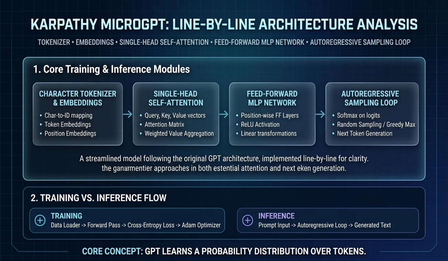
When you open the code to properly understand GPT, surprisingly, the peripherals come out before the essence.
PyTorch, CUDA, tokenizer, dataset loader, optimizer, scheduler, checkpoint, distributed training. In practice, this is a necessary device. But when you first try to figure out “what does GPT actually calculate,” these devices obscure your view.
The reason Andrej Karpathy'smicrogpt.pyis good isn't because it's small. This is because it peels off almost all hidden layers and makes the GPT learning loop visible all the way through in one file. The path starting from the character tokenizer to scalar autograd, Q/K/V attention, negative log likelihood, Adam update, and autoregressive sampling is revealed.
The goal of this article is not to “introduce a small GPT implementation”. The goal is to check what calculations occur behindloss.backward()andoptimizer.step(), why attention is divided into Q/K/V, and what kind of loop the next token learning turns into in the actual code.
microgpt.pyis a short file of around 200 lines. So, rather than avoiding the original text and explaining it, read this article following the flow of the original text, including enough key code blocks and dismantling them right below. It's a safe bet to check back at Karpathy's microgpt.py gist for the most up-to-date source at the time of publication.
Analysis base date: 2026-05-05
Analysis target: Andrej Karpathymicrogpt.pygist
Analysis method: Excerpt of key code blocks following the flow of the original text, explanation by line, connection to GPT structure
Caution: Since the gist can be modified, you must re-check the original revision before actual study or reproduction.
Key takeaways
microgpt.pyshows GPT not as a “library call” but as an execution loop with a computational graph, attention, and optimizer connected.- The key roles of
Tensor,autograd,Module, andoptimizer.step()hidden by PyTorch are directly revealed as small Python objects and lists. - The model is not a large LLM, but a small decoder-only Transformer that learns the name dataset character by character. So the structure is visible, but performance is not the goal.
- Attention is implemented in the following flows:
Q,K,V, scaled dot product, softmax, and weighted sum. This part is the reference point for reading Transformer. - After reading this code, GPT learning can be summarized as “the process of creating a computational graph to increase the probability of the next token and modifying the weight with gradient.”
Note: The code blocks in this article are excerpts to be read along the flow of the original text, which is about 200 lines long. This is not an implementation of GPT for production, but rather a reference for learning.
Order of reading this article
You can read it from beginning to end, but it's faster if you change the viewing order depending on your purpose.
| target | Section to see first |
|---|---|
| I am curious about PyTorch autograd. | Valueclass, local gradient,backward() |
| I’m curious about Transformer attention | Q/K/V generation, multi-head attention, KV cache |
| I am curious about the GPT learning loop. | Next-token problem conversion, loss calculation, Adam update |
| I'm curious about the reasoning. | BOS start, temperature softmax, sampling |
If you want to see only the core flow, you can look in the following order:Value.backward()togpt()to loss calculation to Adam update to sampling.
1. What code ismicrogpt.py?
This code can be defined in one sentence as follows:
Learn a small GPT with a character-level name dataset,A pure Python executable that generates a string that looks like a new name.The original file only uses standard libraries such asos,math, andrandom. The code includes data download, tokenizer configuration, autograd engine, Transformer forward pass, Adam update, and inference sampling, in that order. So this file is less of a “small model” and more of a transparent laboratory for observing GPT execution paths.
| item | detail |
|---|---|
| file name | microgpt.py |
| Author | Andrej Karpathy |
| implementation language | Python |
| External ML dependencies | doesn't exist |
| data | List of names in the formnames.txt |
| tokenizer | Character-by-character tokenizer |
| model structure | Small decoder-only Transformer |
| learning objectives | Next character prediction |
| optimizer | Adam implemented it himself |
| way of reasoning | autoregressive sampling |
The core message is this:
The center of GPT is the calculation that increases the probability of the next token.However, separate system engineering is required to make the calculation quickly and large.2. Entire execution flow
Let's start with the flow of the program.
Check input.txtIf you don't have to, download names.txtCreate a to docs listto create character vocabularyConfigure scalar autograd with to Value classto embed / attention / MLP / lm_head weight initializationTo learn next-token prediction one by one-> loss.backward()parameter update to Adamto Generate character samples starting from BOSThis flow is a microcosm of actual GPT training.
In an actual large model, the dataset is web-scale, the tokenizer is a BPE series, and the computation is performed with a GPU tensor kernel. But the core of the algorithm is still the same.
Convert tokens to vectorsto attention and pass MLPto predict the next token probabilityto create a loss by comparing it with the correct answer.Calculate the to gradientUpdate weight with to optimizerDuring to inference, the next tokens are sampled one by one.3. Import and seed fixation
The first part to look at is import and seed.
import os # os.path.existsimport math # math.log, math.expimport random # seed, choices, gauss, shuffle random.seed(42)These four lines may seem simple, but they show the nature of the code.
| cord | role |
|---|---|
os | Check whether theinput.txtfile exists. |
math | Use mathematical functions such aslogandexp. |
random | Used for data shuffling, weight initialization, and sampling. |
random.seed(42) | Makes the execution results somewhat reproducible. |
The important thing is that there is nonumpy,torch,tensorflow. In other words, this code shows the learning and inference flow of GPT without the tensor library. Instead, all operations occur on Python scalars and lists, so the speed is very slow.
In practice, we don't learn this way. But it's a good form to understand what PyTorch does under the hood.
4. Dataset preparation
Preparing training data looks something like this:
if not os.path.exists('input.txt'): import urllib.request names_url = 'https://raw.githubusercontent.com/karpathy/makemore/988aa59/names.txt' urllib.request.urlretrieve(names_url, 'input.txt') docs = [line.strip() for line in open('input.txt') if line.strip()]random.shuffle(docs)print(f"num docs: {len(docs)}")The original code downloadsnames.txtofmakemoreif there is noinput.txt, reads each line as one document, and creates adocslist.
| step | explanation |
|---|---|
| check file | Check whether the training file exists in the current directory. |
| remote download | If not, download the name dataset. |
| Read line by line | One name is considered one document. |
| Remove blank lines | Exclude meaningless input. |
| shuffle | Shuffle the training sequence under a fixed seed. |
docslooks roughly like this.
["emma", "olivia", "ava", "isabella"]In general GPT learning, when you think of a document, you might think of a long text such as a web page, book, code file, or conversation record. But here, one name is one document.
doc = "emma"This model is not a model that generates sentences, but a character-level GPT that generates strings that look like names.
5. Character-level tokenizer
Next is the tokenizer.
uchars = sorted(set(''.join(docs)))BOS = len(uchars)vocab_size = len(uchars) + 1 print(f"vocab size: {vocab_size}")Sort all unique characters that appear in the dataset, and use the last index as theBOSspecial token.
| cord | explanation |
|---|---|
unique_characters(docs) | Collect the letters that appear in all names. |
sorted(...) | Fixes the character order. |
BOS = len(uchars) | Let the number following the character index be a special token. |
vocab_size = len(uchars) + 1 | Add 1 special token to the number of characters. |
For example, if your dataset only has 26 lowercase letters of the alphabet, it would look like this:
uchars = ['a', 'b', 'c',..., 'z']BOS = 26vocab_size = 27In actual learning, addBOSbefore and after the name.
tokens = [BOS] + [uchars.index(ch) for ch in doc] + [BOS]For example,"emma"is conceptually converted to this:
[BOS, e, m, m, a, BOS]The firstBOSmeans "Now the name begins". The finalBOSis also used to mean "the end of the name."
In practice, tokenizers usually separateBOS,EOS,PAD,UNK, etc. This code uses one special token for both start and end for simplicity.
6.Valueclass and scalar autograd
One of the most important parts of this file is theValueclass.
class Value: __slots__ = ('data', 'grad', '_children', '_local_grads') def __init__(self, data, children=(), local_grads=()): self.data = data # forward value self.grad = 0 # gradient for loss self._children = children # Previous node in the computation graph self._local_grads = local_grads # local derivative for each childThis one object looks like a simple number, but it actually has four pieces of information.
| field | meaning |
|---|---|
data | Actual numeric value calculated in forward pass |
grad | gradient indicating how sensitive the loss is to this value |
_children | Previous nodes used to create this value |
_local_grads | The local derivative of the current node with respect to its children |
By analogy to PyTorch,Valueis a very smallTensor. However, PyTorch Tensor is a multidimensional array, andValueis a single scalar.
| division | Value | PyTorch Tensor |
|---|---|---|
| unit | scalar one | multidimensional array |
| algorithm | Python scalar operations | vectorized tensor operations |
| autograd | implement it yourself | Built-in framework |
| speed | slow | speed |
| purpose | For educational use | Practical learning/reasoning |
Karpathy's separate project, micrograd, is also a small autograd engine that dynamically creates a DAG on scalar values and performs reverse-mode autodiff.
Ultimately, theValueclass ofmicrogpt.pyis a device for answering the following questions:
If loss.backward() isn't magic,What exactly happens inside?7. Addition, multiplication, local gradient
Valuesaves the calculation graph while creating the calculation result as a newValue.
def __add__(self, other): other = other if isinstance(other, Value) else Value(other) return Value(self.data + other.data, (self, other), (1, 1)) def __mul__(self, other): other = other if isinstance(other, Value) else Value(other) return Value(self.data * other.data, (self, other), (other.data, self.data))Starting with addition, the forward value isx + y, and the local gradient is 1 on both sides.
z = x + y dz/dx = 1dz/dy = 1Multiplication is different.
z = x * y dz/dx = ydz/dy = xSo the local gradient of multiplication is the counterpart value.
Thanks to this structure, when you later callloss.backward(), you can obtain the gradient of all parameters by following the calculation graph backwards.
8.backward()and chain rule
The core of autograd isbackward().
def backward(self): topo = [] visited = set() def build_topo(v): if v not in visited: visited.add(v) for child in v._children: build_topo(child) topo.append(v) build_topo(self) self.grad = 1 for v in reversed(topo): for child, local_grad in zip(v._children, v._local_grads): child.grad += local_grad * v.gradThis function can be understood in three steps.
1. Starting from loss, collect the entire computational graph.2. Topologically sort the graph.3. Apply the chain rule by rotating from back to front.The most important line is this:
child.grad += local_grad * v.gradWhen written as a formula, it is as follows:
dLoss/dChild += dCurrent/dChild * dLoss/dCurrentIn other words, it is a chain rule. The principle behind the next line in PyTorch is the same.
loss.backward()The difference is the execution unit. PyTorch processes quickly in tensor units, andmicrogpt.pyprocesses slowly but transparently in units of scalarValueobjects.
9. Initialize model parameters
Now we create parameters for the GPT model to learn.
n_layer = 1n_embd = 16block_size = 16n_head = 4head_dim = n_embd // n_head| setting | value | meaning |
|---|---|---|
n_layer | 1 | Transformer block number |
n_embd | 16 | token embedding dimension |
block_size | 16 | Maximum context length |
n_head | 4 | number of attention heads |
head_dim | 4 | The dimension that one head is responsible for |
These values are extremely small compared to actual LLM. However, the structure retains the basic form of GPT.
embedding-> attention-> MLP-> output logitsThe weight matrix is also filled withValueobjects rather than regular numbers.
matrix = lambda nout, nin, std=0.08: [ [Value(random.gauss(0, std)) for _ in range(nin)] for _ in range(nout)]This way, each weight can have its own gradient after the forward pass.
10.state_dict: Gather GPT components
The parameters are stored instate_dict.
state_dict = { 'wte': matrix(vocab_size, n_embd), 'wpe': matrix(block_size, n_embd), 'lm_head': matrix(vocab_size, n_embd),}| key | role |
|---|---|
wte | token embedding |
wpe | position embedding |
lm_head | Output layer that converts hidden vectors into vocab logits |
The weights inside the Transformer layer have the following characteristics.
| weight | meaning |
|---|---|
attn_wq | query projection |
attn_wk | key projection |
attn_wv | value projection |
attn_wo | attention output projection |
mlp_fc1 | MLP extended projection |
mlp_fc2 | MLP reduced projection |
MLP quadruplesn_embdand then decreases it again.
16 -> 64 -> 16Finally, expand all parameters into a one-dimensional list. This is to make it easier for the optimizer to traverse and update all parameters.
11.linear,softmax,rmsnorm
There are three helpers that are repeatedly used in the model forward.
def linear(x, w): return [dot(row, x) for row in w]This function is a matrix-vector product. When written in PyTorch, it looks roughly like this:
y = W @ xBut here it is not a tensor operation. All multiplication and addition areValueoperations. Therefore,linear()is a simple calculation and at the same time creates an autograd graph.
Next is softmax.
def softmax(logits): max_val = max(val.data for val in logits) exps = [(val - max_val).exp() for val in logits] total = sum(exps) return [e / total for e in exps]softmax turns logits into a probability distribution.
softmax(x_i) = exp(x_i) / sum(exp(x_j))The reason for subtracting the maximum value first here is because of numerical stability. For example, if logits is[1000, 1001, 1002], overflow may occur when applying the exponential function as is. Subtracting the maximum gives[-2, -1, 0], the softmax result is the same, but the calculation is much more stable.
Next is RMSNorm.
def rmsnorm(x): ms = sum(xi * xi for xi in x) / len(x) scale = (ms + 1e-5) ** -0.5 return [xi * scale for xi in x]RMSNorm normalizes values based on the root mean square of the input vector. RMSNorm paper removes the mean-subtracting re-centering in LayerNorm and proposes RMS statistics-based normalization.
12.gpt()function and embedding
Now this is the model body, thegpt()function.
def gpt(token_id, pos_id, keys, values): tok_emb = state_dict['wte'][token_id] pos_emb = state_dict['wpe'][pos_id] x = [t + p for t, p in zip(tok_emb, pos_emb)] x = rmsnorm(x)| cord | meaning |
|---|---|
wte[token_id] | Get the embedding vector of the current token. |
wpe[pos_id] | Get the position embedding of the current location. |
tok_emb + pos_emb | Add token information and location information. |
rmsnorm(x) | Normalizes the input vector size. |
Transformer does not process the token id itself directly. First, change the token id to vector.
token_id -> token embedding vectorHowever, attention alone cannot tell the order of tokens. So, you need to include location information as well.
token embedding + position embedding[Transformer paper] (https://arxiv.org/abs/1706.03762) also explains that in structures without recurrence and convolution, positional encoding is added to input embedding to use sequence order information.
13. Making Q, K, V
When entering the Transformer block, we first prepare attention.
x_residual = xx = rmsnorm(x) q = linear(x, state_dict[f'layer{li}.attn_wq'])k = linear(x, state_dict[f'layer{li}.attn_wk'])v = linear(x, state_dict[f'layer{li}.attn_wv']) keys[li].append(k)values[li].append(v)Q, K, and V are the core concepts of attention.
| name | meaning | intuition |
|---|---|---|
| Query | Information that the current token wants to find | “What do I want to see?” |
| Key | Address or characteristics of each token | “What kind of information am I?” |
| Value | What will actually be delivered | “What do I have to give?” |
keys[layer].append(k)andvalues[layer].append(v)are small KV caches. Because only the key/value up to the current location is accumulated, the model cannot see future tokens.
In a typical decoder-only transformer, a causal mask is used to mask future tokens.microgpt.pyprocesses tokens one by one from left to right rather than inserting the entire sequence at once. So the autoregressive condition holds without an explicit causal mask.
What you can see at your current position:[BOS, previous characters, current character] What you can't see in your current position:future characters14. Deconstructing multi-head attention
Ifn_embd = 16,n_head = 4, the dimension of head is 4.
Full embedding 16 dimensions head 0: 0~3head 1: 4~7head 2: 8~11head 3: 12~15Instead of performing one large attention, we divide the vector into pieces and perform attention from multiple perspectives.
for h in range(n_head): hs = h * head_dim q_h = q[hs:hs+head_dim] k_h = [ki[hs:hs+head_dim] for ki in keys[li]] v_h = [vi[hs:hs+head_dim] for vi in values[li]]The attention score is calculated using the scaled dot-product.
attn_logits = [ sum(q_h[j] * k_h[t][j] for j in range(head_dim)) / head_dim**0.5 for t in range(len(k_h))]attn_weights = softmax(attn_logits)[Transformer thesis] (https://arxiv.org/abs/1706.03762) explains that the dot product of the query and key is divided by the square root of the key dimension and then softmax is applied to create a weight for the value.
Then the values are weighted.
head_out = [ sum(attn_weights[t] * v_h[t][j] for t in range(len(v_h))) for j in range(head_dim)]x_attn.extend(head_out)In other words, attention answers the following questions:
For the current token to predict the next token,Which of the previous tokens should I refer to and how much?15. Attention output and residual connection
After concatenating the results of each head, output projection is performed.
x = linear(x_attn, state_dict[f'layer{li}.attn_wo'])x = x + x_residualThe first line shuffles the output of multiple heads back into the embedding dimension.
multi-head output -> output projectionThe second line is the residual connection.
x = attention_output + original_inputResidual connections help information and gradients flow well in deep networks. Transformer papers also use residual connections around each sub-layer.
Althoughmicrogpt.pyhas only one layer, the structure itself follows the basic pattern of the GPT block.
RMSNorm-> Multi-head Attention-> Output Projection-> Residual Add16. MLP block andlm_head
Attention is followed by an MLP block.
x_residual = xx = rmsnorm(x) x = linear(x, state_dict[f'layer{li}.mlp_fc1'])x = [xi.relu() for xi in x]x = linear(x, state_dict[f'layer{li}.mlp_fc2']) x = x + x_residualIf you write the structure in one line, it looks like this.
x -> RMSNorm -> Linear -> ReLU -> Linear -> Residual AddIn size, it looks like this:
16 -> 64 -> 16If attention determines “which past token to look at,” MLP nonlinearly transforms the hidden representation of each location. The Transformer paper also uses a position-wise feed-forward network in addition to the attention sub-layer.
Finally, it passes through the output head.
logits = linear(x, state_dict['lm_head'])return logitslogitsis not yet a probability.
logits = raw score for next token candidatesFor example, if it isvocab_size = 27, there are also 27 logits. If softmax is applied here, it becomes the next token probability.
probs = softmax(logits)Ultimately, thegpt()function does the following:
Receive the current token, current position, and past KV cacheReturns logits for the next token.17. Learning loop: turning one name into a next-token problem
The learning loop selects one document at each step and creates a token sequence prefixed withBOS.
for step in range(num_steps): doc = docs[step % len(docs)] tokens = [BOS] + [uchars.index(ch) for ch in doc] + [BOS] n = min(block_size, len(tokens) - 1)| cord | meaning |
|---|---|
docs[step % len(docs)] | Select a document. |
encode(doc) | Converts characters to token id. |
[BOS] +... + [BOS] | Append start and end tokens. |
min(block_size,...) | Trim it so that it does not exceed the maximum context length. |
For example,doc = "emma"would be the following sequence.
[BOS, e, m, m, a, BOS]This sequence changes to the following problems during learning.
| input token | Correct answer token |
|---|---|
BOS | e |
e | m |
m | m |
m | a |
a | BOS |
This is the basic goal of GPT learning.
Guess the next token based on the tokens you have seen so far.18. Loss calculation
The forward pass and loss calculations have the following structure.
keys, values = [[] for _ in range(n_layer)], [[] for _ in range(n_layer)]losses = [] for pos_id in range(n): token_id, target_id = tokens[pos_id], tokens[pos_id + 1] logits = gpt(token_id, pos_id, keys, values) probs = softmax(logits) loss_t = -probs[target_id].log() losses.append(loss_t) loss = (1 / n) * sum(losses)The key is the negative log likelihood of the correct answer token probability.
loss = -log(P(correct_next_token))The higher the probability of the correct answer token, the smaller the loss.
P(correct) = 0.9-log(0.9) ~= 0.105If the probability of the correct answer token is low, the loss increases.
P(correct) = 0.01-log(0.01) ~= 4.605In other words, the model is trained to change the weight to give a higher probability to the actual next character.
19.loss.backward(): Flow gradient to all parameters
Once loss is created, backpropagation is performed.
loss.backward()This one line callsValue.backward()created earlier. In reality, we follow the following path backwards:
loss-> log-> softmax-> logits-> lm_head-> MLP-> attention-> embedding-> parametersEach parameter is aValueobject. Therefore, afterloss.backward(), thegradfield of each parameter is filled.
p.gradThis value has the following meaning:
If I change this parameter slightly, how much does the loss change?In practical terms, this perspective is also important when understanding PyTorch'sloss.backward(). This one line isn't magic, it's the process of applying the chain rule by following the computation graph backwards.
20. Direct implementation of Adam optimizer
Now we update the parameters using gradient.
learning_rate = 0.01beta1 = 0.85beta2 = 0.99eps_adam = 1e-8 m = [0.0] * len(params)v = [0.0] * len(params)Adam paper introduces Adam as a stochastic optimization algorithm that uses adaptive estimates of the lower-order moments of the gradient.
| variable | meaning |
|---|---|
learning_rate | Determines how much to move the parameter at a time. |
beta1 | The decay coefficient of the gradient moving average. |
beta2 | Gradient is the decay coefficient of the squared moving average. |
eps | Prevents division by zero. |
m | This is the first moment buffer. |
v | This is the second moment buffer. |
The update proceeds as follows:
1. As the step progresses, the learning rate decreases.2. Update the moving average m of the gradient.3. Update the moving average v of the gradient squared.4. Correct the bias that occurs in the initial step.5. Modify the parameter value directly.6. Initialize gradient to 0.The core of the original update loop is this part.
lr_t = learning_rate * (1 - step / num_steps) for i, p in enumerate(params): m[i] = beta1 * m[i] + (1 - beta1) * p.grad v[i] = beta2 * v[i] + (1 - beta2) * p.grad ** 2 m_hat = m[i] / (1 - beta1 ** (step + 1)) v_hat = v[i] / (1 - beta2 ** (step + 1)) p.data -= lr_t * m_hat / (v_hat ** 0.5 + eps_adam) p.grad = 0The last line is especially important.
p.grad = 0If you do not initialize the gradient, the gradient of the next step will be accumulated in the previous step. In PyTorch, the role is similar to the following code.
optimizer.zero_grad()optimizer.step()21. Inference: Starting from BOS and generating one letter at a time
Once training is complete, a new name is generated.
temperature = 0.5 for sample_idx in range(20): keys, values = [[] for _ in range(n_layer)], [[] for _ in range(n_layer)] token_id = BOS sample = []The creation loop looks like this:
for pos_id in range(block_size): logits = gpt(token_id, pos_id, keys, values) probs = softmax([l / temperature for l in logits]) token_id = random.choices( range(vocab_size), weights=[p.data for p in probs] )[0] if token_id == BOS: break sample.append(uchars[token_id])The creation flow is as follows:
BOSto sample first letterto sample the second letter->...Quit when to BOS appears.temperature controls the randomness of generation.
| temperature | effect |
|---|---|
| lowness | High probability tokens are strongly preferred. The results are stable but can be monotonous. |
| height | Even low probability tokens have a greater chance of being selected. Results vary, but can get weird. |
Here it istemperature = 0.5. Rather than generating something completely random, it gives a stronger preference to characters that the model deems plausible.
22. Revisit the entire structure at once
The overall structure ofmicrogpt.pycan be summarized as follows.
| panel | code element | Meaning of GPT perspective |
|---|---|---|
| data preparation | docs | Study document list |
| tokenizer | uchars,BOS,vocab_size | Convert string to token id |
| autograd | Value | Scalar-based computational graph and gradient |
| parameter | state_dict | Weight to be learned by the model |
| embedding | wte,wpe | Convert token and position to vector |
| attention | Q/K/V projection | Refer to past tokens |
| MLP | mlp_fc1,mlp_fc2 | Convert hidden representation |
| output | lm_head | Generate the following token logits |
| loss | -log(prob[target]) | Objective function to increase the probability of the correct answer token |
| backward | loss.backward() | gradient calculation |
| optimizer | Adam update | parameter modification |
| inference | probability sampling | Next token generation |
If you boil the main point down to one sentence, it's like this.
microgpt.py is an executable anatomy diagram that allows GPT's training and inference to be traced by hand without PyTorch.The differences from the actual LLM should also be clarified.
| item | microgpt.py | Real LLMs |
|---|---|---|
| tokenizer | character unit | BPE, SentencePiece, tiktoken, etc. |
| operation unit | scalarValue | tensor |
| training data | list of names | large corpus |
| model size | Thousands of parameter levels | Parameters available from billions to trillions |
| learning style | Process documents one by one sequentially | batch, distributed training |
| acceleration | doesn't exist | GPU/TPU, fused kernel |
| purpose | For educational use | production or research |
23. What’s especially worth learning from this code?
It would be a shame to see this code as simply a "small GPT implementation". There are three more important learning points: Once these three things are captured, Transformer code written in PyTorch becomes much less opaque.
23.1 Autograd is a computational graph and chain rule
TheValueclass is a miniature version of PyTorch autograd.
Graph creation when forwardingApply chain rule when to backwardto parameter.grad fillIf you see this process in person, the following code will be much clearer.
loss.backward()optimizer.step()optimizer.zero_grad()23.2 Attention is the comparison of Q and K, the weighted sum of V
The core of attention is three lines:
score = q dot k / sqrt(d)weight = softmax(score)output = sum(weight * value)In other words, the current token does not view all past tokens equally, but gives higher weight to the necessary tokens.
23.3 GPT learning is a process of increasing the probability of the next token.
The learning objectives are not complicated.
Guess the next token with the tokens seen so far.loss is the negative log likelihood of the correct answer token probability.
loss = -log(P(correct_next_token))This principle remains a central idea in both small name generation models and large language models.
24. Practical checklist
If you're following the original code directly, it's a good idea to look at it in the order below.
microgpt.py reading checklist [ ] I checked the original gist reference date.[ ] I understand the flow of downloading names.txt when there is no input.txt.[ ] I understood that one docs is one name.[ ] I understand that uchars, BOS, and vocab_size act as tokenizers.[ ] Can explain the difference between Value.data and Value.grad.[ ] I understand how add and multiply store local gradients.[ ] Can explain topological sort and chain rule of backward().[ ] The roles of wte, wpe, and lm_head can be distinguished.[ ] Can explain the roles of Q, K, and V projection.[ ] I understood attention score = q dot k / sqrt(head_dim).[ ] I understand that the keys and values list acts as a small KV cache.[ ] I understand that the MLP block has a 16 to 64 to 16 structure.[ ] The meaning of loss = -log(prob[target]) can be explained.[ ] Adam's m, v, and bias correction can be roughly explained.[ ] I understand what temperature does in inference.25. Q&A
Q1. Is this code really GPT?
Structurally, it is a decoder-only Transformer-based next-token model. However, the size is very small, the tokenizer is in character units, and the training data is also a list of names.
Therefore, it is more accurate to view it as an educational miniature to understand the GPT structure rather than an actual implementation of GPT.
Q2. Why didn't you use PyTorch?
This is because the goal is algorithmic description, not performance.
With PyTorch,Tensor,Module,autograd,optimizerhide a lot of work. In practice, that is an advantage. However, for learning purposes, the internal structure may not be visible.
microgpt.pydeliberately exposes its hidden parts.
Q3. Why isBOSalso used as the end token?
Because of simplification.
In actual tokenizer,BOSandEOSare usually separated. However, since this code deals with the small problem of name generation, it uses one special token for both the start and end.
Q4. There is no causal mask, so why not look at the future token?
This code does not process the entire sequence at once. Each token is processed one by one from left to right, and only the current key/value is stored in the cache.
Therefore, at the current position, the key/value of the future token does not yet exist.
Instead of covering the future with a mask,We proceed without calculating the future at all.Q5. If I grow this code as is, will I get an LLM?
Conceptually, it's the right direction, but it's difficult as is. A real LLM requires the following elements:
large-scale tokenizerLarge dataset pipelinebatch trainingtensor operationGPU/TPU accelerationmixed precisiondistributed trainingcheckpointevaluationserving stackSecurity and cost managementmicrogpt.pyis a code that shows the framework of the algorithm. The practical LLM has a huge system engineering on top of it.
Q6. What is the most important line in this code?
Personally, there are three streams.
child.grad += local_grad * node.gradThis line is the chain rule, the core of autograd.
attention_score = q dot k / sqrt(head_dim)This expression is the core of attention.
loss = -log(P(correct_next_token))This expression shows the next-token prediction learning goal.
26. References and uncertainty
References
- Andrej Karpathy
microgpt.pygist: Contains the GPT learning and inference process in one file in pure Python. - Karpathy
micrograd: A scalar-valued autograd engine that implements reverse-mode autodiff on top of dynamically created DAGs. - Attention Is All You Need: Explains the basic structure of scaled dot-product attention, multi-head attention, residual connection, feed-forward network, and positional encoding.
- Adam: A Method for Stochastic Optimization: Explains the first moment, second moment, and bias correction ideas of Adam optimizer.
- Root Mean Square Layer Normalization: Describes RMS statistics-based normalization and re-scaling invariance.
confirmed facts
- As of confirmation on 2026-05-05, the original gist contains the
microgpt.pyfile, and is displayed asLast active May 5, 2026 01:01on the GitHub Gist page. - The original code includes data loading, tokenizer,
Valueautograd, Transformer forward, Adam learning loop, and inference sampling. - The original code comments explain that this model follows GPT-2, but uses RMSNorm instead of LayerNorm, no bias, and ReLU instead of GeLU.
Author's interpretation
- This code is not an implementation to actually service GPT, but is more of an educational reference to follow the GPT algorithm by hand.
- The
Valueclass is a good starting point for understanding PyTorch autograd. - Attention implementation is not a tensor operation, but a Python list and scalar operation, so it is slow, but the structure is easy to read.
uncertainty
- Since the gist may be modified, you must re-check the original revision before actual learning or reproduction.
- Execution time may vary depending on Python version, CPU performance, and local environment.
- The commentary in this article is based on the original gist structure confirmed on 2026-05-05.
finish
In summary,microgpt.pyis closer to a code that removes unnecessary devices to understand GPT, rather than a code that makes GPT smaller.
Creating a real LLM requires a lot more systems. The tokenizer changes, the training data grows, and batch training, GPU kernel, distributed training, checkpoint, and serving stack are added. However, most of the central flow of GPT is contained within this file.
character to tokentoken -> embeddingembedding -> attentionattention -> MLPMLP -> logitslogits -> lossloss -> gradientgradient -> Adam updateBOS -> sampling -> generated textWhen first reading, it is better to look atValue.backward()before thegpt()function. The reason is simple. The greatest value of this file is not that it “implements a Transformer,” but that it shows how forward computation becomes a graph, and how that graph returns to a gradient.
Then, if you follow the sequence oflinear(),softmax(), attention score calculation, and loss calculation, the entire structure becomes clear. If you understand this code, Transformer code written in PyTorch will no longer look like two magic lines:loss.backward()andoptimizer.step().
댓글
GitHub 계정으로 로그인하면 댓글을 남길 수 있습니다. 댓글은 GitHub Discussions를 통해 운영됩니다.